GW170817: Implications for the Stochastic Gravitational-Wave Background from Compact Binary Coalescences
Plots from the publication
Contents
Figure 1a -- PI Curves and Omega for BBH, BNS, and total backgrounds
% load in data for Omega
tmp=load('omega.dat');
omega.freq=tmp(:,1);
omega.bbh=tmp(:,3);
omega.bns=tmp(:,6);
omega.total.min=tmp(:,8);
omega.total.med=tmp(:,9);
omega.total.max=tmp(:,10);

% load in data for PI curves
tmp=load('pi.dat');
pi.freq=tmp(:,1);
pi.O2=tmp(:,2);
pi.O3=tmp(:,3);
pi.Design=tmp(:,4);

% Poisson uncertainty band
cut1 = omega.freq<= 1500 & omega.freq>=10;
ff1 = omega.freq(cut1);
xx_stat1a = [ff1;flipud(ff1)];
yy_stat1a = [omega.total.min(cut1);flipud(omega.total.max(cut1))];

% text sizes
ts = 16; % text label size
fs = 20; % axes label font size
afs = 16; % axes font size
lw = 2; % line width

% color specifications
ctot = [31,120,180]/256;  % color for total background
cband = [.9,0.9,0.9];     % color for total poisson error band
cbns = [227,26,28]/256;   % color for BNS median curve
cbbh = [51,160,44]/256;   % color for BBH median curve

figure;
hh = axes;
set(hh,'FontSize',afs)
legs = zeros(1,7); % initiate legend array

% plot total background estimates with error bars
legs(5)=fill(xx_stat1a, yy_stat1a, cband, 'DisplayName','Poisson'); hold on
set(gca,'xscale','log');set(gca,'yscale','log');
loglog(omega.freq,omega.total.min,'-','linewidth',lw,'Color', cband);
loglog(omega.freq,omega.total.max,'-','linewidth',lw,'Color', cband);

% plot sensitivity curves
legs(1) = loglog(pi.freq,pi.O2,'k-','linewidth',lw,'DisplayName','O2');
legs(2) = loglog(pi.freq,pi.O3,'k-.','linewidth',lw,'DisplayName','O3');
legs(3) = loglog(pi.freq,pi.Design,'k--','linewidth',lw,'DisplayName','Design');

% plot median BNS
legs(6) = loglog(omega.freq,omega.bns,'Color',cbns,'linewidth',lw,'DisplayName','BNS only');
% plot median BBH
legs(7) = loglog(omega.freq,omega.bbh,'Color',cbbh,'linewidth',lw, 'DisplayName','BBH only');
% plot median total background
legs(4) = loglog(omega.freq,omega.total.med,'Color',ctot,'linewidth',lw,'DisplayName','Total');

% axes limits and labels
axis([10 1000 2e-10 1e-6])
xlabel('Frequency (Hz)','FontSize',fs)
ylabel('\Omega_{GW}','FontSize',fs)
grid on

% font sizes
hh.FontSize = afs;

% legend
leg=legend(legs,'Location','NorthEast');
legend boxoff;
leg.FontSize = ts;

Figure 1b -- Running SNR
% load in data
tmp=load('running_SNR.dat');
total.time=tmp(:,1);
total.snr.min=tmp(:,2);
total.snr.med=tmp(:,3);
total.snr.max=tmp(:,4);

% Poisson uncertainty band
Time = total.time;
y_min = total.snr.min;
y_med = total.snr.med;
y_max = total.snr.max;
X_stat = [Time;flipud(Time)];
Y_stat = [y_min;flipud(y_max)];

% observing times and labels
o1obs = 4; %months
o2obs = o1obs+9; %months
o3obs = o2obs+12; % months
o4obs = o3obs+12; % months
o5obs = o4obs+24; % months

rlabels = {'O1','O2','O3','Near Design','Design'};

% get index for start of each observing run
t1 = find((abs(Time-o1obs)) == min(abs(Time-o1obs)));
t2 = find((abs(Time-o2obs)) == min(abs(Time-o2obs)));
t3 = find((abs(Time-o3obs)) == min(abs(Time-o3obs)));
t4 = find((abs(Time-o4obs)) == min(abs(Time-o4obs)));
t5 = find((abs(Time-o5obs)) == min(abs(Time-o5obs)));

% plot figure

%text sizes
ts = 16;  % text label size
fs = 20;  % axes label font size
afs = 16; % axes font size
ms = 30; % markder size

% color specifications
cband = [.9,0.9,0.9];    % color for total poisson error band
ctot = [31,120,180]/256; % color for total background

figure;
hh = axes;
set(hh,'FontSize',afs);
semilogy(Time,y_med, 'b-', 'linewidth', 2);
hold on;
poisson = fill(X_stat(2:end-1), Y_stat(2:end-1), cband);
semilogy(X_stat(2:end-1), Y_stat(2:end-1), '-','Color',cband,'linewidth',2);
% SNR=1 line
semilogy([0 100], [1 1], 'k--', 'linewidth', 1.5);
% SNR=3 line
semilogy([0 100], [3 3], 'k--', 'linewidth', 1.5);
% SNR=5 line
semilogy([0 100], [5 5], 'k--', 'linewidth', 1.5);
% total background SNR
tot = semilogy(Time,y_med,'Color',ctot,'linewidth',2);

% plot markers for observing runs
plot(Time(t1),y_med(t1),'.','Color',ctot,'MarkerSize',ms)
plot(Time(t2),y_med(t2),'.','Color',ctot,'MarkerSize',ms)
plot(Time(t3),y_med(t3),'.','Color',ctot,'MarkerSize',ms)
plot(Time(t4),y_med(t4),'.','Color',ctot,'MarkerSize',ms)

% font sizes
hh.FontSize = afs;

% labels and legend
xlabel('Observation time (months)', 'FontSize', fs);
ylabel('SNR','FontSize',fs);
leg = legend([tot, poisson], 'total', 'Poisson', 'Location', 'SouthEast');
legend boxoff;
leg.FontSize = ts;
grid on
axis([0 48 1e-3 20])

% labels
tc = ctot; % text color
text(2, 6.25, '5\sigma', 'FontSize', ts);
text(2, 3.75, '3\sigma', 'FontSize', ts);
text(2, 1.25, '\sigma', 'FontSize', ts);
text(1, 5.e-3, rlabels(1), 'FontSize', ts, 'Color',tc);
text(o1obs+1, 2.5e-2, rlabels(2), 'FontSize', ts, 'Color',tc);
text(o2obs+1, 9e-2, rlabels(3), 'FontSize', ts, 'Color',tc);
text(o3obs+1, 1.25, rlabels(4), 'FontSize', ts, 'Color',tc);
text(o4obs+1, 1.9, rlabels(5), 'FontSize', ts, 'Color',tc);
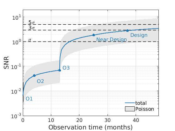
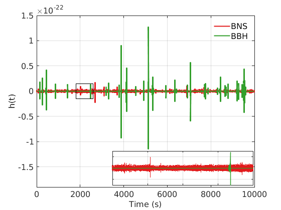
Figure 2 -- Time series for BBH and BNS
% load data

% BNS
tmp=load('bns_time_series.dat');
t1=tmp(:,1)-800000000;
y1=tmp(:,2);

% BBH
tmp=load('bbh_time_series.dat');
t2=tmp(:,1)-800000000;
y2=tmp(:,2);

% plot figure

% text sizes
ts = 16; % text label size
fs = 16; % axes label font size
afs = 12; % axes font size
lw = 2; % line width
lw2 = 1.2; % line width for inset

% color specifications
cbns = [227,26,28]/256;    % color for BNS median curve
cbbh = [51,160,44]/256;    % color for BBH median curve

% plot figure
figure;
hh = axes;
set(hh,'FontSize',afs);

% Adjust XY label font
handxlabel1 = get(gca, 'XLabel');
set(handxlabel1, 'FontSize', fs); %, 'FontWeight', 'bold')
handylabel1 = get(gca, 'ylabel');
set(handylabel1, 'FontSize', fs); %, 'FontWeight', 'bold')

%BNSs
h(1)=plot(t1,y1,'Color',cbns,'LineWidth',lw); hold on;
%BBHs
h(2)=plot(t2,y2,'Color',cbbh,'LineWidth',lw);

% legend
leg=legend(h([1 2]),'BNS','BBH');
legend boxoff;
leg.FontSize = ts;
grid on;
set(gca,'fontsize',fs);
xlabel('Time (s)','FontSize',fs);
ylabel('h(t)','FontSize',fs);

axis([0 10000 -1.9e-22 1.5e-22]);

% inset
% define the region we will show in the inset
inset_xmin=1800;
inset_xmax=2600;
inset_ymin=-1.5e-23;
inset_ymax=1.5e-23;
% plot the rectangle
line([inset_xmin inset_xmax],[inset_ymin inset_ymin],'color','k');
line([inset_xmax inset_xmax],[inset_ymin inset_ymax],'color','k');
line([inset_xmax inset_xmin],[inset_ymax inset_ymax],'color','k');
line([inset_xmin inset_xmin],[inset_ymax inset_ymin],'color','k');

% make the inset
inset_axes = axes('Position',[0.4,0.12,0.5,0.16]); % make axes and set position
plot(t1,y1,'Color',cbns) % plot data
hold on
plot(t2,y2,'Color',cbbh,'LineWidth',lw2);
grid on;
axis([inset_xmin inset_xmax inset_ymin inset_ymax]); % crop it to region we want

% adjust axes properties
inset_axes.XTickLabel = {''};
inset_axes.YTickLabel = {''};